When we want to make sure that the integrity of our safety function is good enough, we use a calculation of probability of failure on demand (PFD) to check against the required reliability level. The requirement comes from a risk analysis as seen up against risk acceptance criteria. But what are we actually calculating, and how do uncertainties and selection of safety intervals change the results?

Most probability calculations are done for the time-averaged value of the probability of failure on demand. Normally we assume that a proof test will discover all failure modes; that is, we are assuming that the test coverage of our proof test is 100%. This may be unrealistic, but for the time being, let us just assume that this is correct. The average PFD for a single component can be calculated as

PFD_avg = λ_DU x τ / 2,

where λ_DU is the failure rate per hour and τ is the proof test interval in hours. Let us now consider what the instantaneous probability of failure on demand is; this value grows with time after a proof test, where it is assumed that the PFD is zero at time zero for 100% proof coverage. The standard model for component reliability follows an exponential distribution. This gives the probability density function for the exponential distribution:

PFD(t) = 1 – e^-λt .

Effect of proof test interval and the time-variation of the PFD value

The instantaneous probability of a failure on demand can thus be plotted as a function of time. With no testing the failure probability approaches one as t → ∞. With the assumption of 100% proof test coverage, we “reset” the PFD to zero after each test. This gives a “sawtooth” graph. Let us plot the effect of proof testing, and see how the average is basically the probability “in the middle” of the saw-tooth graph. This means that towards the end of your test interval the probability of a failure is almost twice the average value, and in the beginning it is more or less zero.

In this example the failure rate is 10^-5 failures per hour and the proof test interval is 23000 hours (a little more than two and a half year). By increasing the frequency of testing you can thus lower your average failure probability, but in practice you may also introduce new errors. Remember that about half al all accidents are down to human errors – several of those during maintenance and testing!

Effect of uncertainty in failure rate data on calculated PFD values

Now to the second question – what about uncertainty in data? For a single component the effect is rather predictable. Let us use the same example as above but we want to investigate what the effect of uncertainty on λ is. Let us say we know the failure rate is between 0.70 and 1.3 times the assumed value of 10^-5. Calculating the same saw-tooth function then gives us this picture:

We can see that the difference is quite remarkable, just for a single component. Getting good data is thus very important for a PFD calculation to be meaningful. The average value for the low PFD estimate is 0.08, whereas for the high PFD estimate it is 0.15 – almost twice as high!

Let us now consider what happens to the uncertainty when we combine two components in series as in this reliability block diagram:

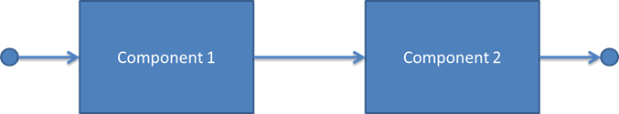
These two components are assumed to be of identical failure rates and with the same uncertainty in the failure rate as above. If both have failure rates at the lower end of the spectrum, we get an overall PFD of PFD₁+PFD₂ = 0.16. If, on the other hand, we look at the most conservative result, we end up with 0.30. The uncertainties add up with more components – hence, using optimistic data may cause non-conservative results for serial connections with many components. Now if we turn to redundant structures, how do uncertainties combine? Let us consider a 1oo2 voting of two identical components.

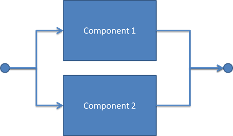
The PFD for this configuration may be written as follows:

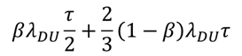
In this expression, which is taken from the PDS method handbook, the first part describes the PFD contribution from a common cause failure in both components (such as defects from production, clogged measurement lines on same mount point, etc.), whereas the second part describes simultaneous but independent failures in both components. The low failure rate value gives a PFD = 0.10, the high failure rate gives PFD = 0.20 and the average becomes 0.15. In both cases the relative uncertainty in the PFD is the same as the relative uncertainty in the λ value – this is because the calculations only involve linear combinations of the failure rate – for more complex structures the uncertainty propagation will be different.

What to do about data

This shows that the confidence you put in your probability calculations come down to the confidence you can have in your data. Therefore, one should not believe reliability data claims without good backup on where the numbers are coming from. If you do not have very reliable data, it is a good idea to perform sensitivity analysis to check the effect on the overall system.